Reduction-based Transformations on Control Flow
Graphs^☆

1. Introduction

A control flow graph (CFG) [1] for a computer program is a graph representing all paths that the program may traverse during its execution. CFGs are central to any static analysis of the flow of execution and data-relationships in a computer program. The use of CFGs in detecting vulnerabilities and malicious behavior in software codes is one such instance [2, 3]. We describe graph transformations on CFGs that reduce its size while retaining essential information for identifying vulnerabilities and malicious behavior in software programs. This reduction can greatly lessen the time for a human analyst to identify such vulnerabilities and malicious behavior in software programs.

Software vulnerabilities and malicious behaviors can be characterized as execution sequences of specific type of events. For example, thread synchronization requires that any two concurrently-executing threads do not execute a common portion of a program at the same time. Use of locks is a commonly used mechanism to ensure thread synchronization. A thread entering a common portion of a program during its course of execution must acquire lock on a mutex object associated with that common portion. We denote the locking event by L(m) for a mutex object m. After executing the common portion the thread must release the lock object so that other concurrently-executing threads are free to execute the common portion in a similar fashion. We denote the releasing event by U(m) (U indicates unlocking) for a mutex object m. To verify safe synchronization of threads it should be checked that in every execution path that contains L(m) for a mutex object m, L(m) is be followed by U(m). A similar analysis can be done for memory leak vulnerability: each allocation of memory for an address a must be followed by the corresponding deallocation for a. A number of vulnerabilities listed in the Common Weaknesses Enumeration by MITRE corporation (http://cwe.mitre.org/index.html) can be modeled by a similar two event characterization.

The two event approach can also characterize malicious behaviors. For example, a common malware activity in smartphone-applications is leaking of a sensitive piece of information to a malicious website [4]. This activity can be modeled as a read event on a sensitive piece of information i, denoted by event R(i), followed by posting i on a malicious website, denoted by event P(i). Thus, a malware-free smartphone application must satisfy the following: on every path in the CFG that has event R(i) for a sensitive piece of information i, R(i) must not be followed by P(i) corresponding to a malicious website.

Verifying software vulnerabilities and malicious behaviors using the above described two event characterization can be computationally expensive because the number of execution paths in CFGs can become exponentially large with the number of non-nested branch nodes [1, 5]. Motivated by this we describe transformation on CFGs that can greatly reduce the size of CFGs while retaining sufficient information to verify the software vulnerabilities. Apart from software vulnerabilities and malicious behaviors, we believe the above described two-event characterization can be useful in modeling other real world problems. For example, consider a computer network covering a large geographic location. It can be represented by a graph, where each node corresponds to a source or a destination computer (or a router). Certain nodes can be vulnerable to attacks and it may be required to add “police” nodes on the network that run tools to scan data packets that have passed through the vulnerable nodes. To verify if police nodes are appropriately placed, every path that has a vulnerable node must have a police node following the vulnerable node. To appeal to such general applicability of CFGs, and not just restricted to static software analysis, we describe our graph transformations in a generic framework of flow graphs. A flow graph is a directed graph G having the following properties:

1. ⊤ (⊥) is a unique node having only outgoing (incoming) edges and is called the entry (exit) node.
2. Every node is reachable from ⊤ and ⊥ is reachable from every node.
3. ℐ is a subset of nodes that are “important”. {⊤, ⊥} ∈ ℐ is always true.

The important nodes are so called because our analysis on flow graphs is focused on the sequence of important nodes in a path in flow graphs. For example, for the analysis of safe synchronization of threads the important nodes correspond to lock and unlock events.

The set of nodes in a flow graph having multiple outgoing edges are called branch nodes. For a flow graph G, V_G, E_G, ℐ_G, ⊤_G and ⊥_G denote the set of nodes, the set of edges, the set of important nodes, the entry node and the exit node of G respectively. We define a flow graph G by the ordered set {V_G, E_G, ℐ_G, ⊤_G, ⊥_G}. When the flow graph G is clear from the context, we drop the subscripts. For two flow graphs A and B, A − B denotes the subgraph of A induced by V_A ∖ V_B. In the subsequent discussion, unless stated otherwise, G denotes a flow graph.

In G, an edge from u (the source node) to v (the destination node) is represented by the ordered pair (u, v). A self-loop in G is an edge of type (u, u) for some node u in G. |G| = |E| + |V| denotes the size of G. Two edges are parallel if they share a common source node and a common destination node.

An end-to-end path in G is a path from ⊤ to ⊥. A trace in G is the sequence of the important nodes encountered in an end-to-end path in G. Two end-to-end paths p₁ and p₂ are equivalent, denoted p₁ ≡ p₂, if they have the same trace. Clearly, ≡ is an equivalence relation over the set of end-to-end paths in a flow graph. The trace content of G, denoted Δ_G, is the set of all traces in G. Let P be the maximal set of end-to-end paths in G such that for any p₁ and p₂ in P, p₁ ≢ p₂. Then, it is easy to see that Δ_G is the union of the traces of all the end-to-end paths in P and |Δ_G| = |P|. That is, |P| represents the minimum number of end-to-end paths that must be considered to evaluate all the distinct traces in G.

2. Graph Transformations

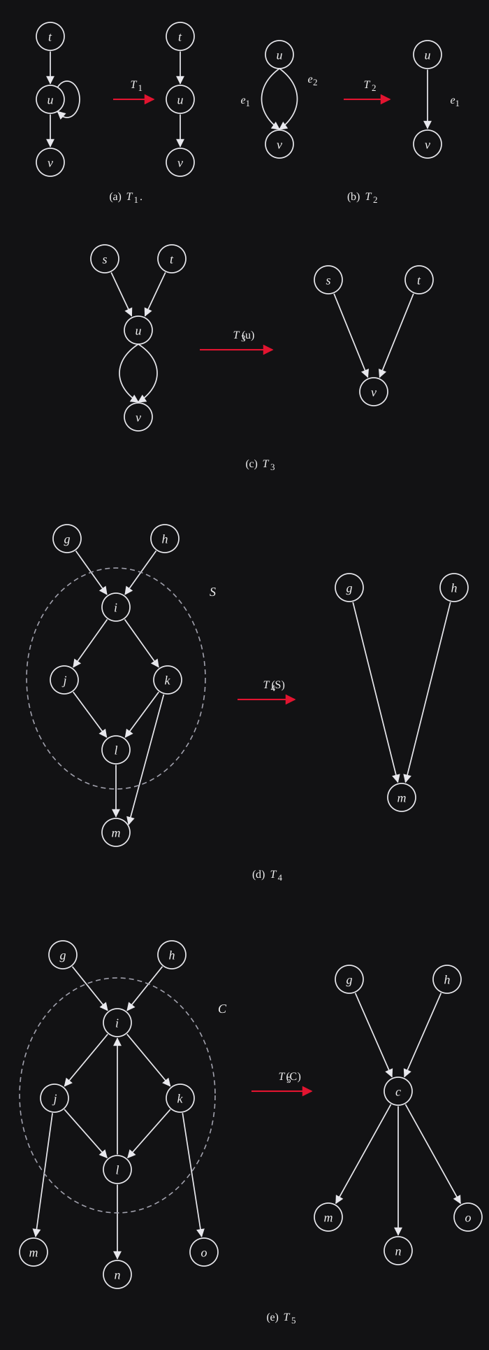
Computing the trace content of a flow graph G can be simplified if the size of G can be reduced while preserving it’s trace content. Motivated by this we describe the following graph transformations.

Type T₁: Transformation T₁ on G removes a self-loop on an unimportant node.

Clearly, T₁ does not change the trace content of G. Figure 1a exemplifies T₁.

Type T₂: Let e₁ and e₂ be two parallel edges. Transformation T₂ on G deletes e₂.

Clearly, T₂ does not change the trace content of G. Figure 1b exemplifies T₂.

Type T₃: Transformation T₃ on G acts on an unimportant node u having all the out-going edges ending in a common node v by deleting all the outgoing edges of u and identifying u into v. Specifically, it does the following:

1. For every edge e = (t, u), delete e and add edge (t, v) to G.
2. Delete u from G.

Clearly, T₃ does not change the trace content of G. Figure 1c exemplifies T₃.

Transformation T₃ can be generalized to a subgraph S of G induced by the unimportant nodes such that all edges from S to G − S end in a common node m. That is, there exists a node m ∈ {V_G ∖ V_S} such that for every edge (u, v) in S, v is in S or v = m. Let such a subgraph be called a single-successor subgraph and m it’s successor node. This motivates transformation T₄:

Type T₄: Transformation T₄ removes a single-successor subgraph S with successor node m such that all the edges incoming to S from G − S now end in m. Specifically, it does the following:

1. For every edge (u, v) in G such that v lies in S and u does not, add edge (u, m) to G.
2. Delete S from G.

Clearly, T₄ does not change the trace content of G. Figure 1d exemplifies T₄. Note that T₃ is a special case of T₄ when the single-successor subgraph consists of a single node. We delay the discussion on how T₄ can be applied on all single-successor subgraphs of G till all graph transformations have been defined.

The intuition behind this transformation can also be applied to strongly connected subgraphs of G induced by the unimportant nodes. Consider a strongly connected subgraph C of G induced by the unimportant nodes. Observe that a path entering C can exit through any of the edges leaving C. Thus, if only the sequence of important nodes on a path is being considered, C acts as a relay point. That is, the trace content of G will not change if C is subsumed by a corresponding relay node. This motivates transformation T₅:

Type T₅: For a maximal strongly connected subgraph C of G induced by the unimportant nodes, transformation T₅ replaces C by a new node c such that all the edges incoming to C from G − C now end in c and all the edges outgoing from C to G − C now start from c. Specifically, it does the following:

1. Add node c to G.
2. For every edge (u, v) in G such that v lies in C and u does not, add edge (u, c) to G.
3. For every edge (u, v) in G such that u lies in C and v does not, add edge (c, v) to G.
4. Delete C from G.

Clearly, T₅ does not change the trace content of G. The desired strongly connected components can be identified in O(|G|) time [6, Section 22.5][7]. Thus, T₅ can be done in O(|G|) time. Figure 1e exemplifies T₅.

2.1. Application of T₄

It is easy to see that if G has no cycles, T₄ can be applied on all single-successor subgraphs in G by repeated applications of T₃ until no longer possible to do so, in O(|G|) time. In case when G has cycles, we check if a node m in G is the successor node to a single-successor subgraph S in G. If such an S exists, T₄ is applied on S. For a node m in G this can be done as show in Algorithm 1.

For any single successor subgraph S with m as its successor node, Algorithm 1 first transforms S into an acyclic graph by maximal application of T₅ on S. It then traverses S in a reverse topological order. The traversal visits any node that has all out going edges in S. Any node that has an out going edge to G − S is never visited. Thus, Algorithm 1 correctly identifies S if it exists. Set 𝒮 in step 2 of Algorithm 1 can be computed in O(|G|) time [6, Section 22.5][7]. Thus, for each node in G Algorithm 1 takes O(|G|) time. Thus, all single-successor subgraphs in G can be identified in O(|G|²) time.

Next, we describe a property of G that allows application of T₄ on all single-successor subgraphs of G in O(|G|) time.

Definition 1. G satisfies property 𝒫 if every maximal strongly connected subgraph C of G induced by unimportant nodes satisfies: If C is not a subgraph of a single-successor subgraph S ≠ C, C has no subgraph C′ ≠ C such that C′ is a single-successor subgraph of G.

If G satisfies 𝒫, T₄ can be applied on all single-successor subgraphs of G in O(|G|) time using Algorithm 2.

In step 3 of Algorithm 2, for a maximal strongly connected subgraph C, it is simple to check in O(|C|) time if C is a single-successor subgraph. Thus, Algorithm 2 takes O(|G|) time. We prove by contradiction that there are no single-successor subgraphs in G after running Algorithm 2. Let S be a single-successor subgraph in G with successor node m after running Algorithm 2. Let S be connected (otherwise we select a connected component of S, which is also a single-successor subgraph). Without loss of generality let S be maximal, i.e., there exists no single-successor subgraph S′ ≠ S of G such that S′ is connected and S is a subgraph of S′. The following two cases are possible:

1. S has no cycles: Thus, S can be topologically sorted. Thus, there exists a node u in S that has no out going edges in S. In G, ⊥ is reachable from every node in S, thus, edge (u, m) exists in G. Thus, T₃ can be applied on u in G — a contradiction!
2. S has cycles: Let S′ be a copy of S. Apply T₅ on all maximal strongly connected subgraphs of S′. Now S′ can be topologically sorted. Thus, there exists a node u in S′ that has no out going edges in S′. If u corresponds to a node in S, for reasons given in the previous case edge (u, m) exists in G. Thus, T₃ can be applied on u in G — a contradiction! If u corresponds to a maximal strongly connected subgraph C of S, C is a single successor subgraph with m as its successor node C. However, C must also be a maximal strongly connected subgraph of G. If this is not the case, there exists a maximal strongly connected subgraph C′ of G such that C′ is not a subgraph of a single-successor subgraph (because S is maximal) and C′ has a subgraph C such that C is a single-successor subgraph. However, this contradicts property 𝒫 of G. Thus, C is a maximal strongly connected subgraph of G. However, C was not identified in steps 2 and 3 of Algorithm 2 —- a contradiction!

Thus, either case leads to a contradiction. Hence proved.

Even when G does not satisfy property 𝒫, Algorithm 2 can be useful. First run Algorithm 2 on G. If the resulting graph has a single-successor subgraph S, S must be a subgraph to a maximal strongly connected subgraph C ≠ S of G because G violates property 𝒫. Thus, to identify the remaining single-successor subgraphs of G, Algorithm 1 needs to be run on only nodes in maximal strongly connected subgraphs of G, and not on all nodes of G.

Motivated by the above graph transformations, we define the trace reduced form (TRF) of G as the flow graph G′ obtained after the repeated application of T₁ − T₅ on G until no longer possible to do so. It is easy to see that the TRF of G can be obtained in O(|G|²) time.

2.2. Retaining Branch Nodes

The branch nodes can add value to the trace of an end-to-end path. Consider a branch node b having n > 1 outgoing edges. Let P be the set of all end-to-end paths that go through b. Any path p in P takes one of the n out going edges at b. This can be seen as p making a choice at b to select one of the n out going edges. Consider paths p₁ and p₂ in P. Let i₁ and i₂ (i₁ ≠ i₂) be the first important node encountered in p₁ and p₂ respectively after crossing b. In such a case it may be important to include in the trace the choice made at b by p₁ and p₂ respectively that led them to different important nodes. To capture this notion of the choice made by a path as it goes through a condition node, we label the outgoing edges of a branch node. Specifically, the n outgoing edges of branch node b are labeled b₁, b₂ . . . b_n respectively. The conditional trace of an end-to-end path p is the sequence of the important nodes and the labeled edges in p.

Retaining all the labeled edges in the conditional trace may not be informative. For example, consider when branch node b is included in a single-successor subgraph S with m as its successor node. Then every path in P has no important node between b and m. Thus, the choice making at b is irrelevant for a path p in P in deciding the important nodes that p will go through after b. Intuitively, the subgraph S induced by the paths in P between nodes b and i¹ is irrelevant in distinguishing the traces of any two paths in P. That is, for any two paths p₁ and p₂ in P, the distinct choices made by p₁ and p₂ at b, irrespective of what the choices are, is irrelevant in determining if p₁ ≢ p₂. Thus, it makes sense to subsume S in i by applying T₄ on S. In a more general scenario, if b has k < n out going edges e₁ = (b, u₁) . . . e_k = (b, u_k) such that u₁ . . . u_k are included in a single-successor subgraph S, choosing among e₁ . . . e_k is irrelevant in distinguishing the traces of any two paths in P. That is, e₁ . . . e_k represent the same choice. Applying T₄ on S will result in k parallel edges from b to m. Then, applying T₂ k − 1 times on these parallel edges will result in only one edge from b to m, which serves as removing the k − 1 redundant choices. Thus, in either case, i.e., when all or a proper subset of the out going edges of b have their destination nodes in a single successor subgraph, the desired reduction is achieved by applying a combination of T₂ and T₄ transformations.

¹ Specifically, S is defined as follows. For a path p in P, let V_p denote the nodes in its sub path from b to i (including b and i). Then, S is the subgraph induced by ∪_p∈PV_p.

Motivated by this, we define the conditional trace reduced form (CTRF) of G as the flow graph obtained after repeated application of T₁ − T₄ on G until no longer possible to do so. The conditional trace content of G, denoted Δ^c_G, is the set of conditional traces in the CTRF of G. It is easy to see that G can be reduced to it’s CTRF in O(|G|²) time.

3. Concluding Remarks

The flow graphs give a generic framework for analyzing software vulnerabilities and malicious behaviors in software code. The important nodes in flow graphs correspond to events of interest, such as locking/unlocking of mutex objects, and, allocation/deallocation at memory locations. The analysis on flow graphs concerns with how these important nodes appear in paths in a flow graph. This sequencing of important nodes in a flow graph is captured by the trace content of the flow graph. The transformations described can greatly reduce the size of flow graphs, and thus the analysis time, while preserving their trace content. For example, we applied these transformations in verifying safe synchronization property in Linux kernel source (v2.6.31). In the ten biggest functions that use some synchronization mechanism, we observed 89.77%, 87.28% and 99.98% reduction in the number of nodes, edges and paths respectively in the corresponding control flow graphs. We hope our results will be helpful to not just static software analysis but to other real world problems as well.

References

- F. E. Allen, Control flow analysis, SIGPLAN Not. 5 (7) (1970) 1–19.
- D. Bruschi, L. Martignoni, M. Monga, Detecting Self-mutating Malware Using Control-Flow Graph Matching, in: R. Buschkes, P. Laskov (Eds.), Detection of Intrusions and Malware & Vulnerability Assessment, vol. 4064 of Lecture Notes in Computer Science, Springer Berlin Heidelberg, 129–143, 2006.
- C. Lattner, V. Adve, LLVM: A compilation framework for lifelong program analysis & transformation, in: Code Generation and Optimization, 2004. CGO 2004. International Symposium on, IEEE, 75–86, 2004.
- Y. Zhou, X. Jiang, Dissecting Android Malware: Characterization and Evolution, in: Security and Privacy (SP), 2012 IEEE Symposium on, 95–109, 2012.
- M. Das, S. Lerner, M. Seigle, ESP: path-sensitive program verification in polynomial time, SIGPLAN Not. 37 (5) (2002) 57–68.
- T. H. Cormen, C. E. Leiserson, R. L. Rivest, C. Stein, Introduction to Algorithms (The Third Edition), The MIT Press, 2009.
- R. Tarjan, Depth-first search and linear graph algorithms, SIAM journal on computing 1 (2) (1972) 146–160.