A High School Algebra Solution for the
Shortest Path Problem

1 Introduction

The shortest path (SP) problem seeks a path between two vertices such that the total sum of edge weights along that path is minimal among all paths in the graph. Applications of the shortest path problem include digital mapping services, supply chain management, robotic path planning, network routing in telecommunication, power grid contingency analysis, circuit design, community detection in social networks, and arbitrage in financial markets.

Existing solutions —most notably Dijkstra [4] and Bellman-Ford [2,3,8] —rely on iterative graph traversal and extensive bookkeeping to maintain distance estimates. While these methods are foundational, they become inefficient or fail under certain conditions.

This paper presents a fundamentally different perspective that invents a novel use of high-school algebra to solve graph problems. The high-school algebra as expounded in [1, 7] is powerful, beautiful, and accessible without getting entangled in complex mathematical definitions and proofs. This algebra is essentially about inventing concepts to make difficult problems tractable. The paper introduces a novel algebraic framework that captures graph problems through simple algebraic equations and finds answers by solving those equations. It is analogous to solving word problems in school. The method is applicable to a variety of challenging graph problems like the SP problem. The fundamental difficulty of “all-paths” problems is that the graphs can have astronomically many paths, and the problem demands that every path be analyzed to find the answer. Algebra offers a powerful way to systematically organize and analyze all paths in a directed graph.

In our algebraic framework, all paths in a directed graph are represented as an algebraic expression whose variables correspond to the graph’s edges. A particular all-paths problem is solved by problem-specific interpretation of algebraic operations and by parsing and simplifying the algebraic expressions. For the SP problem, addition is interpreted as the minimum (p₁ + p₂: addition of path segments between two nodes is the path segment p₁ or p₂, the one with the minimum weight) and multiplication is interpreted as concatenation (p₁p₂: multiplication is concatenation of path segments p₁ from nodes a to b, p₂ from nodes b to c, and the weight of p₁p₂ is the sum of the weights of p₁ and p₂). The model’s efficiency stems from algebraic simplifications. For example, the algebraic factorization produces a compact expression for all paths in a directed graph.

We discuss broader implications and advantages of the algebraic approach for “all-paths” problems, such as the maximum flow problem or the software verification problem. The fundamental difficulty of software verification is that it demands all execution paths be analyzed. Following up on Dijkstra’s vision of software verification [5] and Knuth’s vision of structured programming [6], we discuss a novel algebraic connection for a unified solution approach to challenging problems from different fields and the possibility of employing powerful capabilities of algebra to find efficient and elegant solutions.

Section 2 gives examples to motivate and exemplify the use of algebra to solve directed graph problems, Section 3 gives a formal description of path algebra and its use to construct the algebraic model of paths, Section 4 describes an efficient algebraic SP solution for directed graphs with negative weights and cycles, Section 5 compares the algebraic solution with traditional solutions, Section 6 discusses a broader exploration of the algebraic method, and Section 7 is the conclusion.

2 Motivating Example

We show an example to motivate the following novel ideas:

1. A directed graph can be represented as algebraic equations.
2. The algebraic representation leads to a compact algebraic model of paths in the graph.
3. The compact algebraic model can be used to solve all-paths problems. We illustrate it via the shortest path problem.

2.1 Graph Represented as Algebraic Equations

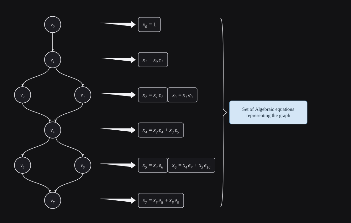
Figure 1 shows a directed graph and the algebraic equations that represent it. There is one algebraic equation for every vertex. A variable x_i is assigned to each vertex v_i; x_i stands for all paths from v₀ to v_i. The variables x_i are unknowns for which we want to get answers.

For each x_i, an equation is set up. The equation for x_i says that the paths to v_i can be obtained from paths to its predecessor v_j. To get a path to v_i, take a path to the predecessor v_j and post-multiply (concatenate) it with the edge from v_j to v_i. Suppose v₁ is the only predecessor of v₂ and e₂ is the edge from v₁ to v₂, then the equation is x₂ = x₁e₂. Suppose v₂ and v₃ are the predecessors of v₄ and e₄, e₅ respectively the edges from the predecessors, then the equation for v₄ is x₄ = x₂e₄ + x₃e₅. Addition stands for union of paths. In other words, x₄ = x₂e₄ + x₃e₅ means the set of paths from v₀ to v₄ is the union of two sets – one is the set of paths from v₀ to v₂ concatenated by e₄ and the other is the set of paths from v₀ to v₃ concatenated by e₅. In Figure 1, you can see that the set of paths from v₀ to v₄ is {e₁e₂e₄} ∪ {e₁e₃e₅}. Note that for the source, a vertex with no predecessors, x₀ = 1. In the algebraic model, ‘1’ denotes an empty path not the number 1.

2.2 Algebraic Model of Paths

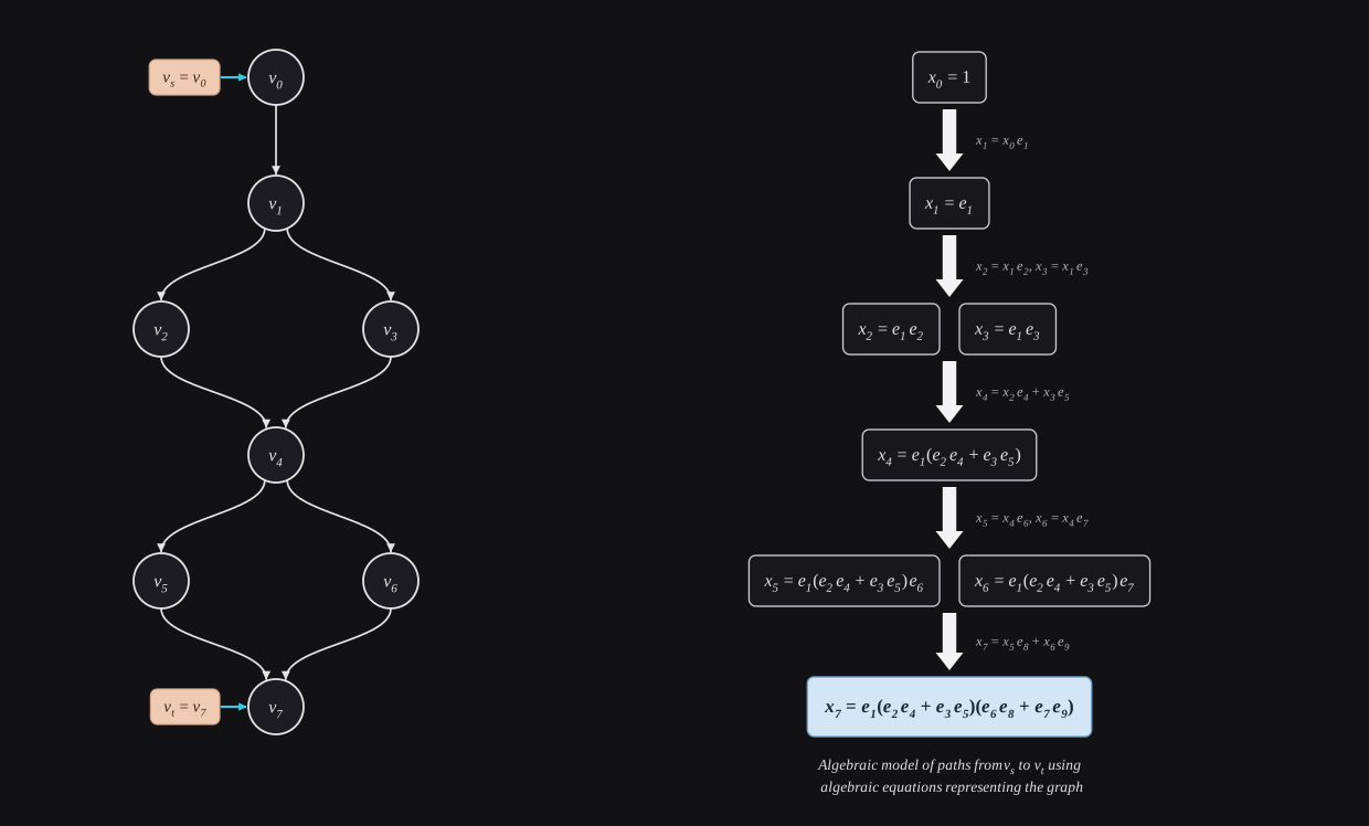
Figure 2 illustrates the derivation of an algebraic expression as a compact algebraic model of paths from a source to a sink. The equations for vertices as set up above (Figure 1) are solved. The resulting answer is an algebraic expression whose variables are the edge symbols e_i. The algebraic expression is the algebraic model of paths. You will see that each term obtained by post-multiplying the subexpressions of the algebraic model gives exactly one path, labeled by its sequence of edges. Every path is uniquely captured by the algebraic model of paths.

In this example, v₀ is the source, v₇ the sink. As shown in Figure 2, the algebraic expression is derived by back substitutions starting at the source. With each sweep of back substitutions, we get the algebraic model for one v_i and finally for v₇. The algebraic expression obtained as the solution for x_i is the model of paths from v₀ to v_i.

The solution x₇ = e₁(e₂e₄ + e₃e₅)(e₆e₈ + e₇e₉) represents all paths from v₀ to v₇. Path are exactly the terms obtained by multiplying the subexpressions. Here the terms are: e₁e₂e₄e₆e₈, e₁e₂e₄e₇e₉, e₁e₃e₅e₆e₈, e₁e₃e₅e₇e₉. In Figure 1, you can see that these terms are exactly the four paths from v₀ to v₇. Each term is one path, labeled by its sequence of edges.

The algebraic expression for all paths is compact because of algebraic factorization. While the number paths can be extremely large compared to the number of edges, the size of the algebraic model of paths remains compact with size proportional to the number edges.

2.3 Shortest Path from Algebraic Model

Given a set of edge weights, we have a corresponding shortest path. We exemplify how to get the shortest path from algebraic model. We do it for two scenarios of weights: in the first scenario all weights are positive, in the second scenario some weights are negative. We chose the two scenarios to relate the algebraic method to Dijkstra’s and Bellman-Ford SP algorithms.

Dijkstra’s SP algorithm does not work for negative weights. Bellman-Ford SP Algorithm works for negative weights but requires significantly more computation than Dijkstra’s algorithm. The algebraic method works for negative weights without the additional computation that Bellman-Ford algorithm requires.

In Dijkstra’s and Bellman-Ford algorithms, the entire computation needs to be repeated when weights change. In contrast, the algebraic method does not repeat bulk of its computation (setting up and solving equations) when weights change. It only repeats the work of substituting edge weights to get the shortest path from the algebraic model. This is an important advantage of the algebraic method in many applications where the weights keep changing. For example, in the digital mapping application where the SP problem is to compute the quickest route, each edge corresponds to a road segment, the time to traverse an edge is the weight for that edge, the weights keep changing as the traffic changes.

A quick observation before we go through the two scenarios of weights. The algebraic model represents all paths. As discussed earlier, we can get each path as an algebraic term. We can get the weight for each path by adding the weights for the edges in the path. Then, we can select the path with the minimum weight. Here, x₇ = e₁(e₂e₄ + e₃e₅)(e₆e₈ + e₇e₉) represents the four paths: p₁: e₁e₂e₄e₆e₈, p₂: e₁e₂e₄e₇e₉, p₃: e₁e₃e₅e₆e₈, p₄: e₁e₃e₅e₇e₉ from v₀ to v₇. By adding the weights for the edges in each path, the weights for the paths p₁, p₂, p₃, p₄ are respectively 16, 14, 26, and 24. The shortest path is p₂ with weight 14, the minimum among all paths. This process finds the shortest path, but it is grossly inefficient. In the scenarios below, we hint at a significantly more efficient method to find the shortest path. One point is to avoid computing the weight of each path separately. You can ponder on the crucial role the algebraic simplification plays in computing the shortest path in the two scenarios in Figures 3 and 4. The most efficient algebraic method is formally described later.

2.3.1 Scenario 1: Shortest path with positive weights

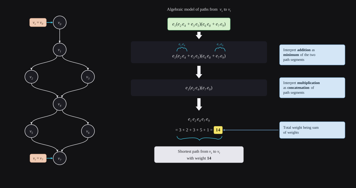
Figure 3 demonstrates how to obtain a shortest path with positive weights. The weights are: e₁: 3, e₂: 2, e₃: 8, e₄: 3, e₅: 7, e₆: 6, e₇: 5, e₈: 2, e₉: 1. The weights are substituted for the edges. The SP problem is solved by interpreting addition as selecting the minimum weight term. and multiplication as concatenation and adding the weights.

Let’s work it out using some algebraic simplifications. First, add weights 2 and 3 to get the weight 5 for e₂e₄. Similarly get the weight 15 for e₃e₅. Then, replace (e₂e₄ + e₃e₅) by the minimum weight term e₂e₄. Similarly, e₆e₈ has weight 8, e₇e₉ has weight 6, so replace (e₆e₈ + e₇e₉) by the minimum weight term e₇e₉. Now, for x₇ = e₁(e₂e₄ + e₃e₅)(e₆e₈ + e₇e₉), we get e₁e₂e₄e₇e₉ – it is the shortest path with weight 3 + 5 + 6 = 14. Note that it is the same as the earlier answer, but now we did less work.

2.3.2 Scenario 2: Shortest path with negative weights

Figure 4 demonstrates how to obtain a shortest path with negative weights. The weights are: e₁: 3, e₂: 2, e₃: 8, e₄: 3, e₅: −7, e₆: 6, e₇: 5, e₈: −2, e₉: 1.

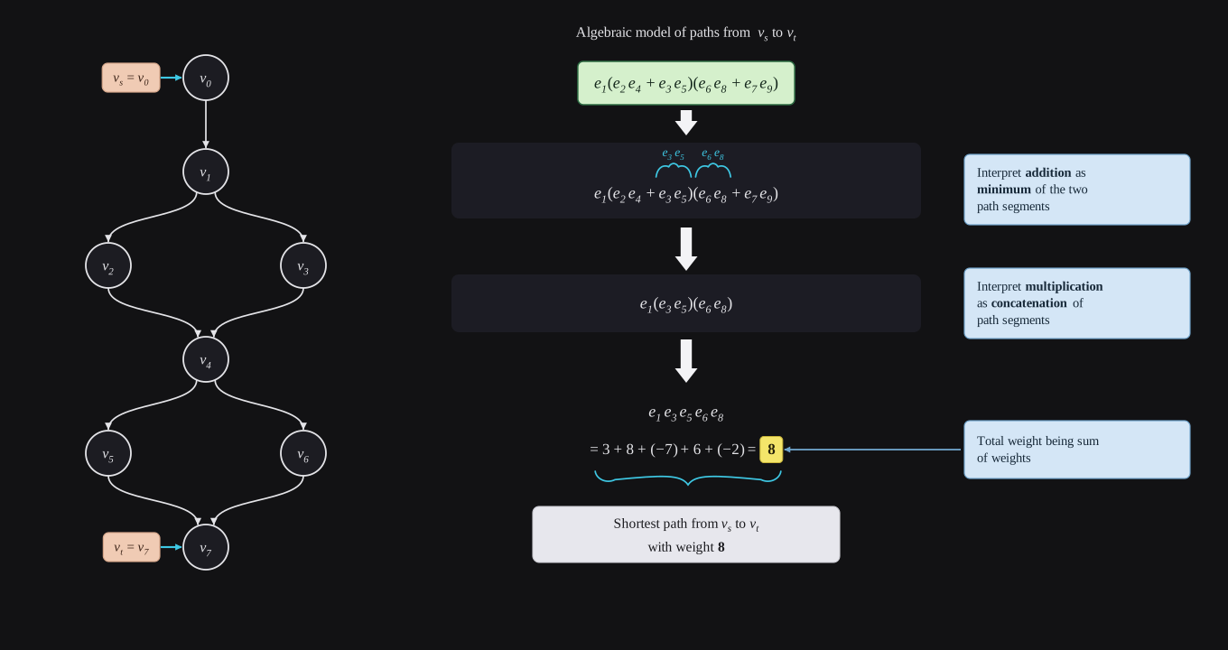
In the algebraic method there is no difference – negative weights are handled the same as the positive weights. Replace (e₂e₄ + e₃e₅) by the minimum weight term e₃e₅ which has weight 1. Replace (e₆e₈ + e₇e₉) by the minimum weight term e₆e₈ which has weight 4. Now, for x₇ = e₁(e₂e₄ + e₃e₅)(e₆e₈ + e₇e₉), we get e₁e₃e₅e₆e₈ – it is the shortest path with weight 3 + 1 + 4 = 8.

Note that with the algebraic model, the same procedure works for both, positive or negative weights.

3 Path Algebra and Algebraic Model of All Paths

The motivating example conveys the intuition for the algebraic model of paths, its use and construction. A formal description is given here by introducing the path algebra.

3.1 Path Algebra

Path algebra is defined on path segments of a directed graph.

In path algebra, an algebraic expression E represents a set of path segments. Addition of two algebraic expressions E₁ + E₂ is the union of the sets of path segments. Multiplication of two algebraic expressions E₁E₂ is the set of path segments p_αq_β where p_α is a path segment in E₁ and q_β is a path segment in E₂. Multiplication of path segments is concatenation of segments. Multiplication is not commutative. One must be careful in maintaining the proper order in multiplication. So, an equation x₂ = x₁e₂ (as in Example 1) cannot be changed to x₂ = e₂x₁. Nor can the solution x₂ = e₁e₂ be changed to x₂ = e₂e₁.

For addition and multiplication in an algebraic model, the path segments have some restrictions. This is similar to the size restrictions on addition and multiplication of matrices. For addition p₁ + p₂, p₁and p₂ must have the same beginning vertex and the same ending vertex. For multiplication p₁p₂, the ending vertex of p₁ must be the beginning vertex of p₂. For example, consider an algebraic model E₁(E₂ + E₃)E₄. All path segments in E₁ end in the vertex A at which path segments in E₂ and E₃ begin. All path segments in E₂ and E₃ end in the same vertex B at which all path segments in E₄ begin. Note that the construction of the algebraic model by setting and solving equations for each vertex ensures that these restrictions for the addition and the multiplication of path segments are satisfied.

Like the Kleene algebra of regular expressions [9] (and in general the algebraic structure called the ring), addition and multiplication in path algebra are associative. Path algebra is a semiring because its elements (path segments) do not have an additive inverse. Path algebra has the important property of the ring – multiplication is distributive over addition. This property enables factorization which is critically important for forming compact algebraic models of all paths. For example, a fully populated binary tree of depth n would have 2ⁿ paths from root to leaves. We could represent all 2ⁿ paths with an expression with only 2n terms, essentially n∏i=1(e_i,1 + e_i,2).

3.2 Algebraic Model of Paths

The algebraic model of paths is for rooted directed graphs. The model is important as a compact representation of all paths from the root (called the source) to each node of the graph. Problems that require analyzing all paths (e.g., the SP problem, the maximum flow problem) can be solved efficiently because the model provides a compact representation and algebraic simplifications to solve the problem.

Definition: For a directed graph G with vertices v₀ (source), v₁, v₂, … , v_t, the algebraic model for G is a set of path algebra expressions E₁, E₂, … , E_t where E_i represents the set of paths from v₀ to v_i.

Constructing the Algebraic Model of Paths

1. Set up the linear equations for the graph.
2. Perform the back substitutions to solve the equations.

Setting up the Linear Equations

Assign a variable x_i to each node v_i; x_i stands for all paths v₀ to v_i. Let k(i) denote the number of predecessors of v_i. Set up the equation for each x_i as follows. Let v_{i 1}, v_{i 2}, … , v_{i k(i)} be the predecessors of v_i, and e_{i j} be the edge from v_{i j} to v_i. The equation for x_i is: x_i = k(i)∑j=1 x_{i j}e_{i j}.

The equation for x_i denotes that the paths to v_i are the paths to each of its predecessors v_{i j} post-multiplied (concatenated) by the edge e_{i j} from the predecessor v_{i j} to v_i.

The equation for v₀ is x₀ = 1.

Solve Equations by Back Substitutions

To solve for x_i, back substitute the path expression obtained as the solution for each predecessor v_{i j} of v_i. Let E_{i j} be the path expression obtained as the solution for v_{i j}. By back substitution the solution for x_i is x_i = k(i)∑j=1 E_{i j}e_{i j}.

The back substitutions start with x₀ = 1. Each back substitution requires k(i) operations to solve for x_i, where k(i) is the number terms in the equation for x_i.

3.3 Detecting Cycles During Back Substitutions

A cycle is a path on which a node gets repeated. As an example, the path ABCABCD is path from node A to D with cycle ABC. This path implies that there must be two edges from C: e₁ going to A to create a cycle, and e₂ going to D which is outside the cycle ABC.

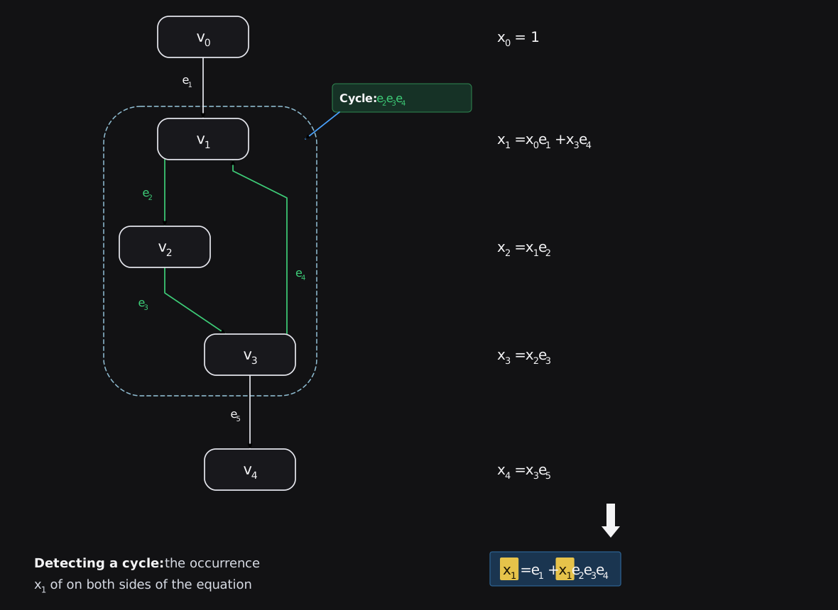
Cycles can be detected while performing the back substitutions as follows. A cycle occurs because a predecessor v_{i j} to v_i has v_i as an ancestor. Then, back substitution results in an equation in which the same variable occurs on both sides of the equation, i.e., x_i = Exp1 + x_iExp2. A cycle is detected when back substitutions lead to an equation in which a variable occurs on both sides of the equation.

Figure 5 exemplifies a cycle and how it is detected. By back substitutions, we get x₁ = e₁ + x₁e₂e₃e₄ in which x₁ is on both sides indicating a cycle.

4 Efficient Algebraic SP Solution

The algebraic model can be customized to make it more efficient for a particular problem. We discuss the customization for the SP problem.

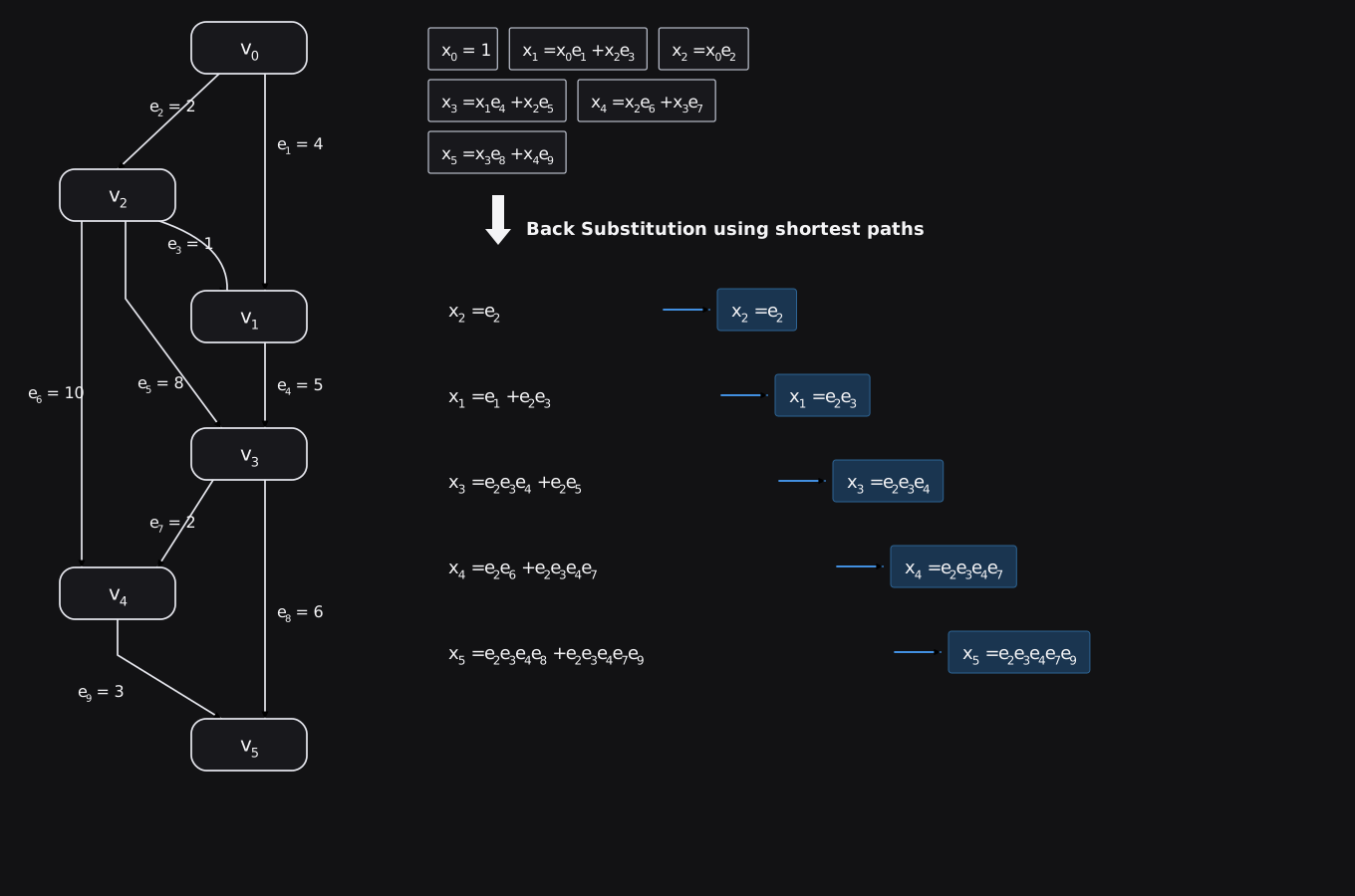
The SP customization is as follows. Note that the algebraic expression x_i = E_i represents all paths from the source to v_i. Before back substituting E_i, we can derive from E_i the subexpression S(E_i) for SP and back substitute S(E_i) instead of E_i.

In deriving SP, multiplication of paths is concatenation of paths and addition of weights and addition of paths is the path with the minimum weight. For example, E_i = ∑_j E_{i j} and the subexpression E_{i 1} gives SP then we back substitute E_{i 1}. The customization is illustrated in Figure 6.

Let V be the number of vertices and E be the number of edges. This efficient algebraic solution has time complexity proportional to E. The algebraic solution has two steps, and the time complexity of each step is proportional E as discussed below.

Time Complexity of Setting up Equations: For each vertex v_i, the equation is x_i = k(i)∑j=1 x_{i j}e_{i j} where x_{i j} are the variables for the predecessors v_{i 1}, v_{i 2}, …, v_{i k(i)} of v_i, and e_{i j} the edge from v_{i j} to v_i. Since each edge e occurs exactly once as e = e_{i j} in exactly one equation, the totality of edges corresponds exactly to the totality of x_{i j}e_{i j} terms across all equations, i.e. V∑i=1 k(i) = E. Intuitively, there are V equations, one for each vertex. Each equation has one term per edge entering its vertex. If the average number of such edges per vertex is E/V, then the algorithm must do work proportional to V ∗ E/V, or simply E. Thus, the time complexity of setting up equations is proportional to E.

Time Complexity of Back Substitutions: As discussed in the customized algebraic SP solution (see Figure 6), back substitutions progress successively by obtaining the SP p_{i j} for each predecessor v_{i j}, of a vertex v_i and substituting p_{i j} for x_{i j} in the equation x_i = k(i)∑j=1 x_{i j}e_{i j}. This substitution augments p_{i j} by e_{i j}, and involves one addition to compute the weight of the augmented path. The SP or v_i is determined by k − 1 comparisons between k augmented paths. Thus, back substitution step x_i = k(i)∑j=1 x_{i j}e_{i j} that computes SP for x_i requires k(i) additions and k(i) − 1 comparisons. Since V∑i=1 k(i) = E, the total number of additions is E and the total number of comparisons is V∑i=1(k(i) − 1) = E − V.

Thus, the overall complexity of the efficient algebraic SP solution is proportional to E. In dense graphs, E is proportional to V². In practical applications, the graphs are sparse, i.e., E is proportional to V.

5 Algebra vs. Traditional Graph Traversal Solutions

We discuss why the algebraic solution is better than Dijkstra [4] and Bellman-Ford [2,3,7] solutions. We compare the solutions for directed graphs with positive or negative weights. Dijkstra solution handles undirected graphs, but it does not work for negative weights. Bellman-Ford handles negative weights, but it does not work for undirected graphs with negative weights. Note that an undirected edge with a negative weight is a negative cycle. Bellman-Ford cannot find shortest simple paths if there is a negative cycle. To the best of our knowledge, the shortest simple path (SSP) problem has remained unsolved for undirected graphs with negative weights.

5.1 Minimal Work for the Source to Sink SP Problem

First, some observations to point out that the minimal work is proportional to E for the source to sink SP problem for directed graphs with negative weights.

Observation 1: There are directed graphs with positive edge weights for which it is necessary to examine each edge at least once to find SP.

Example 1: Here is a simple demonstration of Observation 1. Let G be a directed graph with two distinct paths e_{1 1}e_{1 2} … e_{1 k} and e_{2 1}e_{2 2} … e_{2 k} from the source to the sink. All edge weights are 1. It is necessary to examine each edge at least once to find SP in G.

Observation 2: There are directed graphs with positive edge weights for which it is possible to find SP without examining all edges.

Example 2: Here is a simple demonstration of Observation 2. Let G be a graph with two distinct paths e_{1 1}e_{1 2} … e_{1 k} and e_{2 1}e_{2 2} … e_{2 k} from the source to the sink. All edge weights are 1 except e_{2 1} has weight k. Here it is possible to find the SP e_{1 1}e_{1 2} … e_{1 k}, without examining edges e_{2 2} to e_{2 k}.

Observation 3: For directed graphs with negative edge weights, it is always necessary to examine each edge at least once to find SP.

Dijkstra’s solution can fail for graphs with negative weights because depending on weights it may not examine all edges.

Example 3: Let G be the same as in Example 2 and the weights are the same except e_{2 k} has weight −k. Dijkstra’s solution would find e_{1 1}e_{1 2} … e_{1 k} as SP and not examine edges e_{2 2} to e_{2 k}. Dijkstra gets an incorrect SP. The correct SP is e_{2 1}e_{2 2} … e_{2 k}.

5.2 Algebra vs. Dijkstra

Time complexity of Dijkstra’s solution is proportional to E + V [8]. As discussed in Section 3, time complexity of the algebraic solution is proportional to E, more efficient than Dijkstra.

Dijkstra’s Solution can fail for negative weights. The algebraic solution can handle negative weights. The algebraic solution is optimal, it requires E concatenations and E additions which is the minimal work required to handle negative weights. Dijkstra’s solution works for undirected graphs with positive weights. The algebraic method is not applicable to undirected graphs.

As noted in the motivating example, the algebraic method has an important advantage over Dijkstra’s algorithm in applications where the shortest path has to be recomputed repeatedly because the weights change. In the algebraic method, the bulk of the work, setting and solving equations, is not repeated for different weights. In contrast, in Dijkstra’s algorithm, the entire work has to be repeated when weights change.

5.3 Algebra vs. Bellman-Ford

Bellman-Ford algorithm handles negative weights, but to do so it requires significantly more computation than Dijkstra algorithm. The algebraic method handles negative weights without more computation. Time complexity of Bellman-Ford solution is proportional to EV [8]. Time complexity of the algebraic solution is proportional to E, significantly more efficient than Bellman-Ford.

As noted in the motivating example, the algebraic method has an important advantage over Bellman-Ford algorithm in applications where the shortest path has to be recomputed repeatedly because the weights change. In the algebraic method, the bulk of the work, setting and solving equations, is not repeated for different weights. By contrast, in Bellman-Ford algorithm, the entire work has to be repeated when weights change.

6 Broader Exploration of Algebra

We expect that the applicability and advantages of the algebraic method to extend far beyond the SP problem. Some important capabilities of the algebraic method are not needed in the SP problem because it is less complex. In our ongoing exploration, we find that the maximum flow problem presents the next level of complexity and beyond it are more complex problems of analyzing control and data flow in software. We expect to find novel efficient algebraic solutions to these complex problems. In this section we share our understanding of advantages and extensibility of the algebraic method with the hope that others would be interested in exploring and advancing the algebraic method.

6.1 Structure-Aware Computing with Algebraic Factorization

Algebraic factorization captures the structure of a graph and makes it possible to build a compact model of all paths. The algebra can also act as a filter to separate structural abnormalities.

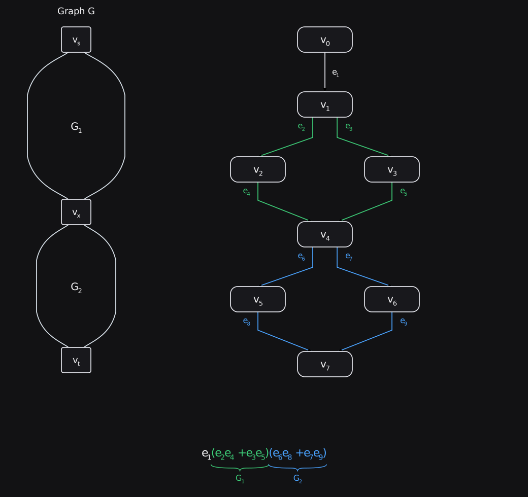
Let’s show by an example how algebraic factorization captures the structure. Figure 7 (a) shows a graph G which is composed of two subgraphs G₁ and G₂. It is like G = G₁G₂, i.e., G can be factored as G₁ followed by G₂. G has the source v_s and the sink v_t. G₁ has the source v_s and the sink v_x. G₂ has the source v_x and the sink v_t. Solving a problem (e.g., SP problem, maximum flow problem, etc.) for G becomes solving two smaller problems one for G₁ and the other for G₂. By combining the solutions for G₁ and G₂ gives the solution for G. For instance, SP for G is p₁p₂ where p₁ and p₂ are respectively the shortest paths for G₁ and G₂.

The structural decomposition of a graph can overcome the astronomical growth in the number of paths which can be a computational barrier. Denote the number of paths in G, G₁ and G₂ by m, m₁, and m₂ respectively. In G, one computes for m = m₁m₂ paths from source to destination. By employing the decomposition, one computes for m₁ + m₂ paths. The astronomical growth in the number of paths is because of the multiplicative effect of subgraphs. The computational barrier of astronomically many paths can be sidestepped by deploying the decomposition.

Algebraic factorization is exactly the mathematical gadget to deploy the structural decomposition of a graph. Figure 7(a) illustrates how the algebraic factorization corresponds to the structural decomposition. It is interesting that the algebraic factorization we study in high school becomes a powerful technique for efficient computation on graphs. In Figure 7(a), note that the two graph substructures are reflected as two subexpressions in the algebraic factorization.

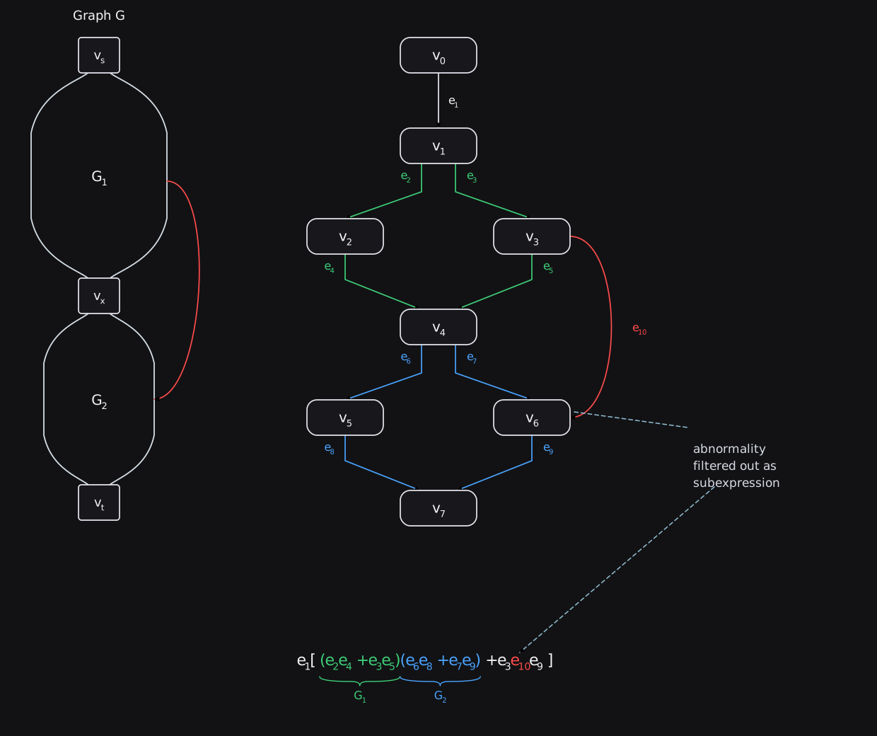
There is another subtle but important advantage of the algebraic factorization. It is to filter out structural abnormalities that obscure the decomposition. This is illustrated in Figure 7(b) where the structural decomposition is obscured by the edge e₁₀. Note that the factorization separates the abnormality caused by the edge e₁₀ with its adjoining edges e₃ and e₉.

6.2 Structured Programs, Structured Graphs, and Algebraic Factorization

In an article titled Structured Programming with go to Statements [6], Knuth writes:

“The real issue is structured programming, but unfortunately this has become a catchphrase whose meaning is rarely understood in the same way by different people. Everybody knows it is a Good Thing, but as McCracken has said, “Few people would venture a definition. In fact, it is not clear that there exists a simple definition as yet.” Only one thing is really clear: Structured programming is not the process of writing programs and then eliminating their go to statements.”

Knuth goes on:

“Indeed, Dijkstra’s original article which gave Structured Programming its name never mentions go to statements at all; he directed attention to the critical question, “For what program structures can we give correctness proofs without undue labor, even if the programs get large? By correctness proofs he explained that he does not mean formal derivations from axioms, he means any sort of proof (formal or informal) that is “sufficiently convincing”; and a proof really means an understanding.”

You may be wondering what does the algebraic method got to do with structured programs. We can point to a very interesting connection. Imagine the graphs in Figure 7(a) and 7(b) to be control flow graphs. The program for the graph in Figure 7(a) would be “structured” written with two consecutive if statements. The graph in Figure 7(b) needs a go to statement for the edge e₁₀. Interestingly, a structural abnormality in graph corresponds to a programming statement considered unstructured.

We conjecture a mathematical notion of “structured graphs” parallel to the notion of “structured programs.” Following Dijkstra’s intuition [5], software verification could be simpler for programs whose control flow graphs are structured. Software verification needs analysis of all execution paths. So also, for other graph problems that need analysis of all paths, the solution could be simpler if the graph is structured. In a forthcoming paper, we will show a simpler and more efficient algebraic solution for the maximum flow problem when the graph is structured.

In our ongoing work we are pursuing an interesting characterization for structured graphs: a directed graph with one source and one sink in which every node is on some path from source to sink is structured if and only if every edge appears exactly once in the optimally factored algebraic model of all paths from the source to the sink. As a corollary, a structured program could then be characterized as one whose control flow graph is structured.

Note that for the graph in Figure 7(a), every edge appears exactly once in the algebraic model: e₁(e₂e₄ + e₃e₅)(e₆e₈ + e₇e₉). For the graph in Figure 7(b), some edges appear multiple times in the algebraic model e₁[(e₂e₄ + e₃e₅)(e₆e₈ + e₇e₉) + e₃e₁₀e₉]. We can try other factorizations for the graph in Figure 7(b), but in every factorization some edges would always be repeated. Maximum repetitions occur with no factorization where the algebraic model of all paths is simply the addition of all paths: e₁e₂e₄e₆e₈ + e₁e₂e₄e₇e₉ + e₁e₃e₅e₆e₈ + e₁e₃e₅e₇e₉ + e₁e₃e₁₀e₉. We encourage the reader to set algebraic equations and solve them to obtain the algebraic model for the graph shown in Figure 7(b). It would be similar to the work shown for the motivating example in Section 2. The reader can also watch the video [11] where the graph, the equations, and the algebraic model are derived by an automated tool that takes a C program as input.

Using algebra, efficient solutions can be developed for specific problems as we have done for SP problem. However, there is a need to explore a general theory of algebraic solutions for all-paths graph problems. Note that there are multiple ways to factorize an algebraic expression. A promising avenue is the general theory of factorization including its optimality and its use to derive efficient solutions to challenging graph problems where the fundamental challenge is astronomically many paths.

7 Conclusion

The paper presents a novel SP solution for directed graphs. It handles negative weights and negative cycles. The time complexity for Dijkstra is proportional to E + V, for Bellman-Ford it is proportional to EV, and for the new solution it is proportional to E. The novel solution detects negative cycles.

The following SP problems are unsolved to the best of our knowledge.

1. Directed Graphs: Find the shortest simple path when negative cycles are present.
2. Undirected Graphs: Find the shortest simple path when some edge weights are negative.

We think that the proposed algebraic solution can be extended to solve the first problem. The algebra is currently not defined for undirected graphs, and thus it requires a non-trivial extension to address the second problem. Contrary to claims on discussion forums (e.g. [10]), Bellman-Ford cannot solve the second problem. Since an undirected edge with a negative weight is a negative cycle, Bellman-Ford would detect negative cycle but not find the shortest simple path.

Besides solutions to a specific graph problem, we introduce an alternative to the graph traversal method used by traditional algorithms. The alternative is a very different perspective in which graph problems are solved by algebra. This new perspective is inspired by our training in high school algebra using Chrystal’s classic algebra book [1], and the valuable lessons from Abhyankar and Hironaka’s great strides in algebraic geometry using high-school algebra – a topic on which Abhyankar reflects in [7].

We expect that the applicability and advantages of the algebraic method to extend far beyond the SP problem. Some important capabilities of the algebraic method are not needed in the SP problem because it is less complex. In our ongoing exploration, the next level of complexity is seen in the maximum flow problem, and beyond it are even more complex software control and data flow problems for which we expect novel efficient solutions using algebra. Algebra changes the way we can reason about software and offers an opportunity to perform software verification as envisioned by Dijkstra [5] and Knuth [6]. Software verification is a pressing need to avert catastrophic safety and cybersecurity failures. The fundamental challenge is the need to analyze astronomically many execution paths. Even with a few hundred lines of code the number of execution paths can be larger than the estimated number of atoms in the universe. Algebra, by the virtue of factorization, offers the capability to construct and manipulate a compact model of all paths. A compact model of all paths is a dire necessity for large-scale software verification.

We think there is a need to explore a general theory of algebraic solutions. A promising avenue is the general theory of factorization including its optimality and its use to develop a new generation of algebraic solutions for challenging graph problems that come up in different applications.